Thomas.I Microsoft BI & Analytics

A Site Dedicated to General BI Issues and MS BI Issues: Architecture and Technology

DAX Code Snippet: Year To Date in Charts

Posted by thomasivarssonmalmo on June 3, 2015

This short blog post tries to show the different ways to solve the same problem in DAX and in MDX.

If you look at the picture you can see two ways of presenting a year to date value. The last picture continues with the last value for all empty months. The example is from measuring database file sizes over time. The charts are made in Power BI Designer.


Two diagrams with accumulated values

The last chart is simple to create in DAX:

TotalYTDSize = TOTALYTD(SUM(‘DW AssesmentDatabaseFileSizes'[size]),’DW DimDateExt'[DateID])

What about the first chart? I had to do a search and found the result in the MSDN new group about DAX but not in DAX books.

TotalYTDSize2 = IF(ISBLANK(SUMX(‘DW AssesmentDatabaseFileSizes’,’DW AssesmentDatabaseFileSizes'[size])),BLANK(),TOTALYTD(SUM(‘DW AssesmentDatabaseFileSizes'[size]),’DW DimDateExt'[DateID]))

The interesting part is that you need a DAX table function, SUMX, because SUM will not work.

What about the same problem in MDX? I am using the know Adventure Works cube instead and show the result in a grid.

With Member Measures.YTDOrderQty AS
SUM(YTD([Date].[Calendar]),[Measures].[Internet Order Quantity])

Member  Measures.YTDOrderQtyAdj AS
IIF(ISEMPTY([Measures].[Internet Order Quantity]),NULL,SUM(YTD([Date].[Calendar]),[Measures].[Internet Order Quantity]))

Select {[Measures].[Internet Order Quantity],Measures.YTDOrderQty,Measures.YTDOrderQtyAdj} On 0,
Descendants([Date].[Calendar],[Date].[Calendar].[Month]) on 1
FROM [Adventure Works]

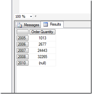
And here is the result in the grid. It is the last column that works like the first chart above.

MDX Result

Posted in DAX Time Calculations, MDX for everyone | Tagged: | Leave a Comment »

Migration from Time Intelligence Dynamic Named Sets in BISM MD To Tabular Models

Posted by thomasivarssonmalmo on March 27, 2015

If you read my previous post about migration from named sets in BISM MD to an attribute based approach, with current flags, inside the BISM MD model this is pretty straight forward. By the way it works fine with Power View in SharePoint and DAXMD. How do we migrate these named sets in BISM MD to Power Pivot, BISM Tabular with DAX?

The same views as in the previous post should be part of the model.

The Power Pivot Model

This is the model in Power Pivot.

PowerPivotModel


To this model you need to add one DAX Time calculation.

ParallelPeriodOrderQty:=CALCULATE(SUM(FactInternetSalesUpdate[OrderQuantity]);SAMEPERIODLASTYEAR(DatesPlus5Y[FulldateAlternateKey5Y]))

Note that the name of this calculation is ParallelPeriod but in DAX we do not use the DAX ParallelPeriod() function. You will have to use SamePeriodLastYear() instead.

Attribute Relations?

No you do not have to think about that. Only add the current flags to the model.

Excel 2013 Pivot Tables with Power Pivot

This is how the report with a current flag set to Y for the Current12Months attribute.

PivotTable


What about Power View?

The current flags works fine in Excel 2013 Power View as well. Note the filter set to Current12Months = Y. The row axis is correct and the calculations.

PowerView


The model will also work in Power View for SharePoint and DAXMD.

Posted in BISM TAB & MD | Tagged: , , | Leave a Comment »

Dynamic YearMonth Axis With Current Flags and the Importance of Attribute Relations in BISM MD

Posted by thomasivarssonmalmo on March 26, 2015

In my previous post I had a TSQL script to move the Adventure Works DW database to current dates. The second idea was to create attribute members that point to CurrentDate, CurrentMonth and Current12Months. The reason for this is that named sets in BISM Multidimensional(BISM MD) are not supported in Tabular and Power Pivot. Named Sets are also not part of the DAXMD that integrates Power View for SharePoint with an external BISM MD model. So why not try to create attributes that might succced Named Sets?

Create the Current Members With TSQL

From my previous blog post I have made a little change and added distinct to the view. The reason is that we had a leap year in 2008 that will create two copies of 2013-02-28. One from the real date and one from the leap year date. Here I move the date dimension five years forward.

CREATE View [dbo].[DateDimensionUpdate]
As
(
Select Distinct
DATEADD(YEAR,5,FullDateAlternateKeY) as FulldateAlternateKey5Y,
DATEDIFF(MONTH,DATEADD(YEAR,5,FullDateAlternateKeY),GetDate()) as MonthSequence,
DateName(m,DATEADD(YEAR,5,FullDateAlternateKeY)) As MontName,
DatePart(m,DATEADD(YEAR,5,FullDateAlternateKeY)) As MontNbr,
Year(DATEADD(YEAR,5,FullDateAlternateKeY)) as Year5,
Year(DATEADD(YEAR,5,FullDateAlternateKeY))*100 + Month(DATEADD(YEAR,5,FullDateAlternateKeY)) As YearMonth5,
Year(DATEADD(YEAR,5,FullDateAlternateKeY))*100 + Datepart(qq,DATEADD(YEAR,5,FullDateAlternateKeY)) As yearQty5,
Case When DATEADD(YEAR,5,FullDateAlternateKeY)  = Convert(varchar(8),GetDate(),112) Then ‘Y’ Else ‘N’ End As CurrentDate,
Case When DATEDIFF(MONTH,DATEADD(YEAR,5,FullDateAlternateKeY),GetDate()) = 0 Then ‘Y’ Else ‘N’ End as CurrentMonth,
Case When DATEDIFF(MONTH,DATEADD(YEAR,5,FullDateAlternateKeY) ,GetDate())between 0 and 2 Then ‘Y’ Else ‘N’ End as CurrentThreeMonths,
Case When DATEDIFF(MONTH,DATEADD(YEAR,5,FullDateAlternateKeY) ,GetDate())between 0 and 5 Then ‘Y’ Else ‘N’ End as CurrentSixMonths,
Case When DATEDIFF(MONTH,DATEADD(YEAR,5,FullDateAlternateKeY) ,GetDate())between 0 and 11 Then ‘Y’ Else ‘N’ End as Current12Months,
Case When DATEDIFF(MONTH,DATEADD(YEAR,5,FullDateAlternateKeY) ,GetDate())between 0 and 23 Then ‘Y’ Else ‘N’ End as Current24Months,
Case When DATEDIFF(MONTH,DATEADD(YEAR,5,FullDateAlternateKeY) ,GetDate())between 11 and 23 Then ‘Y’ Else ‘N’ End as Current12MonthsLY
From [dbo].[DimDate]
)

The second view is required to move one of the fact tables 7 years ahead.

Create View [dbo].[FactInternetSalesUpdate]
AS
(
Select
    CustomerKey,
    ProductKey,
    DATEADD(YEAR,7,OrderDate) As OrderDate,
    DATEADD(YEAR,7,ShipDate) As ShipDate,
    DATEADD(YEAR,7,DueDate) As DueDate,
    OrderQuantity
from [dbo].[FactInternetSales])

I assume that you know how to add these views to a new BISM MD project.

The BISM MD model

Here is the structure of the model that is a simplified version of the Adventure Works cube with only one fact table and with only Order Quantity as the fact table measure.

Simple Cube

Here is the dimension usage tab for the cube.

Dimension Usage


The Date Dimension

Here are the attributes and a hierarchy.  I started with this and added the attribute relations for the hierarchy. I assume that you know about how to map each attribute to type properties and value column properties.

The Date Dimension


The Mistake

After building the cube with the dimensions and the simple fact table I thought I was close to a working solution where I can use the current flags to do selections of YearMonth members and that MDX calculations will work. I started in Management Studio to create some session based calculations with time intelligence.

WITH Member Measures.ParallelPeriodOrderQty AS
SUM(ParallelPeriod([Order Date].[Year Month5].[Year Month5],12,[Order Date].[Year Month5]),[Measures].[Order Quantity])

Select {[Measures].[Order Quantity],Measures.ParallelPeriodOrderQty} On 0,
[Order Date].[Year Month5].[Year Month5] On 1
From [AdventureWorksDW2012Simple]
Where ([Order Date].[Current12 Months].&[Y])

The problem with this MDX query is that it works fine with all parts except if you include the slicer part in the Where clause. The ParallelPeriodOrderQty will be null with slicer. The correct months will appear on the row axis however. So what did I forget to add in the cube?

Attribute Relations

Remember the date dimension picture above. We had  a hierarchy and the matching attribute relations for the hierarchy. Here is what solved my problem. The solution was to add the current attributes as attribute relations to the Year Month5 attribute as you can see in the picure.


AttributeRelations


After adding these attribute relations to the date dimension I runned this query with this result:

TheSolution

Problem solved. Attribute relations are very important in BISM MD. Also you have dynamic flags that will update each time you process the cube and you do not have to use named sets. This solution will also work in Power Pivot as you will se in the next blog post.

Posted in End users dilemma with SSAS structures | Tagged: , | Leave a Comment »

Update Adventure Works with views

Posted by thomasivarssonmalmo on March 16, 2015

Here are two scripts to create two views in the Adventure Works DW database so that you can play around with current dates instead of having to go back several years.

First the date view:

Create View dbo.DatesPlus5Y

AS

(

Select

DATEADD(YEAR,5,FullDateAlternateKeY) as FulldateAlternateKey5Y,

DATEDIFF(MONTH,DATEADD(YEAR,5,FullDateAlternateKeY),GetDate()) as MonthSequence,

DateName(m,DATEADD(YEAR,5,FullDateAlternateKeY)) As MontName,

DatePart(m,DATEADD(YEAR,5,FullDateAlternateKeY)) As MontNbr,

Year(DATEADD(YEAR,5,FullDateAlternateKeY)) as CalendarYear,

Year(DATEADD(YEAR,5,FullDateAlternateKeY))*100 + Month(DATEADD(YEAR,5,FullDateAlternateKeY)) As YearMonth,

Year(DATEADD(YEAR,5,FullDateAlternateKeY))*100 + Datepart(qq,DATEADD(YEAR,5,FullDateAlternateKeY)) As YearQuarter,

Case When DATEADD(YEAR,5,FullDateAlternateKeY) = Convert(varchar(8),GetDate(),112) Then ‘Y’ Else ‘N’ End As CurrentDate,

Case When DATEDIFF(MONTH,DATEADD(YEAR,5,FullDateAlternateKeY),GetDate()) = 0 Then ‘Y’ Else ‘N’ End as CurrentMonth,

Case When DATEDIFF(MONTH,DATEADD(YEAR,5,FullDateAlternateKeY) ,GetDate())between 0 and 2 Then ‘Y’ Else ‘N’ End as CurrentThreeMonths,

Case When DATEDIFF(MONTH,DATEADD(YEAR,5,FullDateAlternateKeY) ,GetDate())between 0 and 5 Then ‘Y’ Else ‘N’ End as CurrentSixMonths,

Case When DATEDIFF(MONTH,DATEADD(YEAR,5,FullDateAlternateKeY) ,GetDate())between 0 and 11 Then ‘Y’ Else ‘N’ End as Current12Months,

Case When DATEDIFF(MONTH,DATEADD(YEAR,5,FullDateAlternateKeY) ,GetDate())between 0 and 23 Then ‘Y’ Else ‘N’ End as Current24Months,

Case When DATEDIFF(MONTH,DATEADD(YEAR,5,FullDateAlternateKeY) ,GetDate())between 11 and 23 Then ‘Y’ Else ‘N’ End as Current12MonthsLY

From [dbo].[DimDate])


And then a fact table view. Feel free to add the measures you need. I have added flags for current date, month , year and so on, to replace named sets that do not work in n Tabular and Power View DAXMD.

Create View dbo.FactInternetSalesUpdate

AS

(

Select

CustomerKey,

ProductKey,

DATEADD(YEAR,7,OrderDate) As OrderDate,

DATEADD(YEAR,7,ShipDate) As ShipDate,

DATEADD(YEAR,7,DueDate) As DueDate,

OrderQuantity

From [dbo].[FactInternetSales])

The MD cube or the Tabular model need a Daily process so that the current flags will be accurate. Thanks to MVP Peter Larsson.

Posted in BISM TAB & MD, Power View, PowerPivot and DAX | Tagged: | Leave a Comment »

MS BI On Premises 1999-2015

Posted by thomasivarssonmalmo on January 6, 2015

This is an attemp to ge a overview of all the software and versions within the MS BI stack  since 1999.  Look at the first column to get the SQL Server version and look to the right on each row to see what has been added over time. My personal view is that it became hard to know each tool really good with the arrival of SQL Server 2005 and it became even harder when SharePoint came as the portal part. I have also tried to identify versions when there has beeen important Changes over SQL Server versions like SSIS in SQL Server 2012. Interesting is that the MS BI certification pays most attention to the SQL Server RDBMS with two exams. I agree that the TSQL part is important but not the other, administration in the context that a lot of BI software is not covered.


MSBI On Premises

Posted in MS BI Platform | Tagged: , | Leave a Comment »

BIG MAC Index with Power Map and Power View

Posted by thomasivarssonmalmo on May 27, 2014

The Big Mac Index is an invention by the news magaziine “The Economist” to measure if a countrys currency is over or under valued. One way to do this is to use the prize of the Big Mac in USD as a comparative product since it is the same all over the world. Then take the price of the Big Mac in all local currencies and calculate that local price into the USD price and compare it to the USD-price. You can read more here.

So what I have done is that I have imported the data from The Economist, in several Excel spreadsheets and used Power Query to change data types and did some minor corrections. Only a few countries have continous data from 2000 to 2014 and a lot of the world countries are not part of the index.

Power Map

Above is the state in early 2014. Since US is the comparative country nothing will show up there. Over valued countries and currency are entirely dark blue. Undervalued countries and currencies have white edges. According to the map Norway, Swiitzerland, Sweden and Venezuela have the most overvalued currencies.

Here is a recording of the tour  where you can see the development over 14 years.


We can also have a look at Norway in Power View.

Power View

As I can say, from several stays in Norway it is a really expensive country and  beatyful. Norway stays at the top during most years.

Posted in Power Map, Power View | Tagged: , , | Leave a Comment »

My BI Year 2013

Posted by thomasivarssonmalmo on January 1, 2014

I had too little time to blog as much as I wanted. The one about SSAS evaluation nodes was the one that took me a lot of time to write and it should have a second part with more practical stuff but there was simply no time for that in 2013.

So what happened then? I can mention the word certification.  I took both the 70-463, implementing a data warehouse with SQL Server 2012, and the 70-461, querying MS SQL Server 2012 and I am currently preparing for the 70-462, administering MS SQL Server 2012 databases. The two last ones, from my point of view as a BI consultant, are a waste of time. I am very happy to have passed the 70-463, because it is very useful in my daily work. Parts of the TSQL certification are useful, like 30-40 percent but I would like to see a more BI-focused database engine part with admin and TSQL parts in one exam. Right know both exams are too developer and DBA focused. The goal is to get the MCSA title, since it is mandatory in the company that I work for. It will not make me better as a BI-consultant since I never do cluster installations, Always On installation or set up replication of the database engine. Most of my customers either has outsourced maintenance of hardware and software or would never let me play with their IT-infrastructure. I have colleagues that have these skills and do this work daily.

The parts of BI that have have spent most of my time on, the last ten years, like Reporting Services and BISM MD/Tabular come in the second certification step, to be a “MS Certified Solutions Expert.

Now to the other parts. The year was mostly spent on the ETL or ELT part of BI. I have been involved in name standard document for BI like clening up that the same term applies to different objects or different terms apply to the same object. I was also invloved in discussions with customers about ETL or ELT strategies.

I attended a 5 day long course on the new PDW V2 and that hardware and software solution really can compete on the high data volume scenarios of BI. Do not think about it as only a part of the BIG Data scenarios because it can integrate well with SQL Server environments without the BIG data part. My personal opinion is why you should invest in more than 4 socket CPU system because on the declining return on adding more CPU power. This also questions the Fast Track part of MSBI offerings since PDW V2 gives much better value for money.

I also worked with a POC for a customer that included SQL Server 2012, BISM Tabular, SharePoint 2013 and Excel 2013. The fun part was to load a 340 million record fact table in to  a dedicated tabular server and see that it worked very well and that compression worked to shrink data to 15 percent of the original size.

I met a very smart customer that maintain their own business catalog with product and customer definitions outside of their ERP system. When they upgrade their ERP system they use this business catalog with cleaned product- and customer keys. That is what I call true master data management.

Slowly the interst for more self service is riising here in Sweden.  Since Power Pivot requires quite capable hardware like 64 bit laptops with 8 GB RAM and SSD and Office 2013 that will be an investment for most organizations that requires approval since most laptops are still 32 bit with 2-4 GB RAM. On top of that a SharePoint infrastructure is also needed.  Still the idea that IT provides datasets to users that then use Excel 2013 with Power Pivot and perhaps Power Query is attractive since it will reduce pressure on IT to help with data mash up.

Posted in BI Architecture, BISM TAB & MD, Excel 2013 | Tagged: | 1 Comment »

Alternative to drill through in Excel 2013-Quick Explore

Posted by thomasivarssonmalmo on November 24, 2013

I sometimes get feedback on features from customers that I did not recognized when testing the feature on your own. Quick Explore in Excel 2013 is such a feature.

When we build BI solutions and start to deliver data in a tool customers usually would like to validate the data against referenced transactions in the source system. BISM Tabular and BISM Multidimensional both have a feature for this called drill-through but you have limited control over what will be presented.

I start with a Pivot Table in Excel 2013 that use a multidimensional cube but it will work the same in Tabular. You probably recognize the Adventure Works multdimensional  cube.

StartUpPivotTable

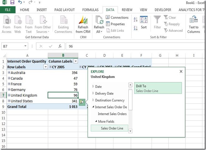
I the next step I will highlight the CY 2005 and United Kingdom cell that tells that the order quantity was 96. You will see a small magnifier glass appear to the right of the cell. That is Quck Explore.

QuickExplore

Qlick on that icon and a small window will open up. I have choosen to go down drill to Internet Sales Order Details –> Sales Order Line to get the reference numbers.


DrillToQE

The result might seem disappointing first since we will se all years of order quantity for United Kiingdom not only 2005.


UK for all years

This issue can be quickly fixed by moving years from columns in the report to the report filter box.


MoveDateToFilters

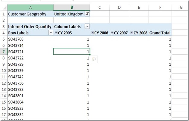
Finally we have a clean list will the sales order numbers for United Kingdom and the year 2005. It is a clean list without any other redundant information.


EndResult

In a Tabular or Multidimensional model you will need to creat a 1-1 dimension with the fact table refered to as a degenerate dimension and in large fact table scenarios this can be a performance problem.

Happy Quick Explore!

Posted in BISM TAB & MD, Excel 2013, OLAP klients | Tagged: | Leave a Comment »

BISM MD: Introduction to Evaluation Nodes

Posted by thomasivarssonmalmo on June 21, 2013

This is the first introduction to the concept of evaluation nodes in SQL Server Profiler and what they can tell you about what is going on in the SSAS engine. I would also like to examine where the evaluation nodes show up in the Profiler trace. Evaluation nodes were introduced as events in SQL Server Profiler with the SQL Server 2012 release. They have been part of the engine before that but it is in the SQL Server 2012 edition they were added as Profiler Events.

I must acknowledge Akshai Mirchandani, from Microsoft, who has answered my questions and given me feedback on this text. If anything is wrong here, blame me.

SSAS/BISM Multidimensional Query Plans

SSAS produces query plans like the SQL Server RDBMS when receiving queries and before doing any real physical work and retrieve data. Query plans in multidimensional structures are complex and would require many chapters in a book to cover. It is not possible to go into all details about how this works in SSAS/BISM MD in this blog post. I refer to the Analysis Services 2008 unleashed for details.
There are two main parts that works in this process and that is the Formula Engine (FE), which does most of the work, except for going to the disk system and retrieve data. A simplified general picture is that the FE handles the MDX (queries) sent to SSAS and breaks that request down into small parts, called sub cubes. It then tries to find out if it can find the data in the FE cache or will have to send it further to the Storage Engine.
Retrieving actual data from disk or the file system cache is the work handled by the other part, the Storage Engine (SE) unless there is data cached in the FE.

Logical and Physical Query Plans

The SSAS FE creates both logical and physical query plans. The SE has its own query plans and it is not a part of this blog post. The word plan here is not fully accurate since the profiler trace shows how the query was executed and not a planned query execution. SQL Server RDBMS query optimizer use estimated query plans and actual query plans but that is not the fact for SSAS/BISM MD.

Evaluation nodes are essentially nodes in the logical plan. Instead of using the word logical query plan it is recommended to use Evaluation node. They get converted into nodes in the physical plan and might get executed. Evaluation nodes can be created but not always executed. They can also be cached and used by other cells during query execution. All of this takes place in the Formula Engine.

Physical plan nodes in the FE implement calculation operations like multiplication and division but nothing of that are exposed in the profiler trace events for evaluation nodes.

Can Evaluation Nodes help in Query Execution Analysis?

Evaluation nodes are chatty events like most SQL Server Profiler Trace events for SSAS/ BISM MD. A lot of data gets generated and not in a friendly User Interface. With more complex calculations than this example you can get a lot of Evaluation Node events that can be hard to find patterns in. This blog post can help you with seeing how the Evaluation Nodes appears as three groups of events, one group that will get executed and two that will not get executed. The post will also help you to find the xml-tags with interesting information about the query plan.

An example of interesting information is if evaluation node is run in cell by cell mode or block mode. Have a look at the table at the end of this blog post where several xml-tags in an evaluation node are explained.


The cube used and the queries

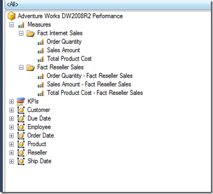
This is my sample cube with two measure groups (no calculations or measure expressions). It is the same cube that I used in my previous blog post.

The Cube Structure

There are no natural or user hierarchies’ only attribute hierarchies. Each MG has only one partition. There are no MDX scripts and no aggregations. The aggregation property of each attribute are set to default.

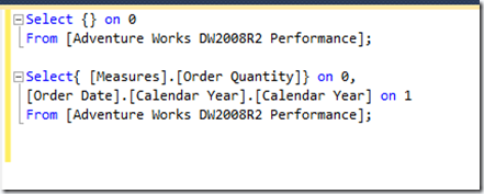
This is the first query that was executed on a non-cached cube.

The MDX Query

Below is the result of the simple query above.

The result of the MDX Query

The Complete Profiler Trace

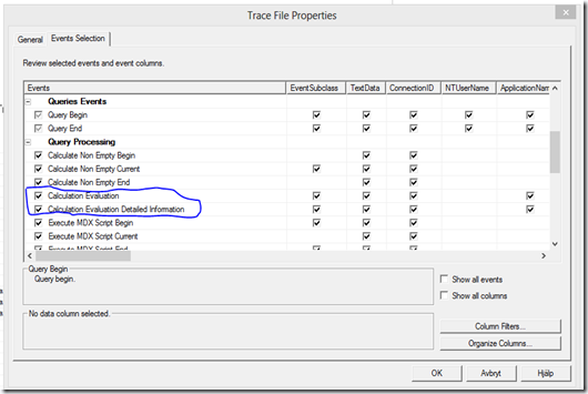
To set up the trace with Profiler you need to add these events before running the query above.

ProfilerTraceSettings

I assume that the reader know how to configure the SQL Server Profiler.

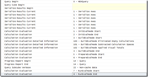
Here is the first part of the Profiler Trace events.

FirstPartProfilerTrace

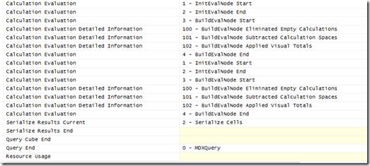
This is the second part of the profiler with the event following the last event above.

SecondPartProfilerTrace

Grouping the Trace Events

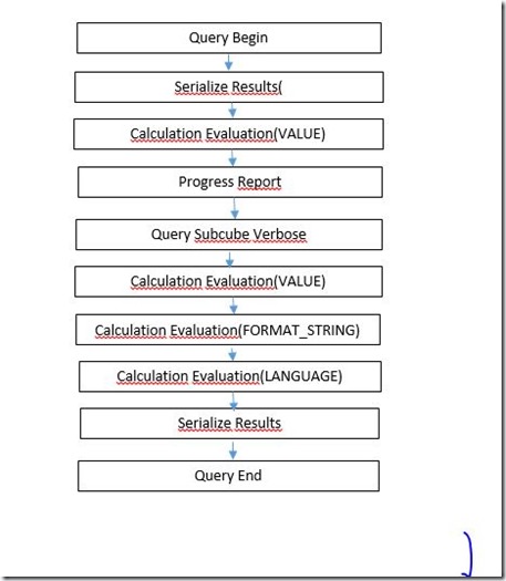
Let me first try to describe what is going on here with a high level picture.

EvaluationNodesTopView

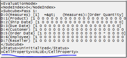
The VALUE, FORMAT_STRING and LANGUAGE groups are derived from an xml-tag (CellProperty) in each evaluation node events that will be shown later. Each group of evaluation nodes have their own NodeIndex-property. The first group starts with NodeIndex 0.

EvalNodesNodeIndex

First the FE starts with analyzing the sets on each axis and builds subcubes that covers these sets. Then an iteration over the cells starts with a request of the current cells property value. Each intersection of axis sets points to a cell. FE will then find a subcube that was previously built and then create an evaluation node for that subcube. This will trigger the Init-Build-Prepare of the evaluation node in the Profiler trace. Data is then requested from the SE that is needed by this evaluation node, including data needed by other evaluation nodes (look at the Query Subcube Verbose event in the Profiler Trace), that were created indirectly by the Build/Prepare phases. Now it is time to run the evaluation node (event 7, RunEvalNode Start and 8, RunEvalNode End). This is optional sometimes since because evaluation nodes do not always have to be run (for non-value cell properties or cell-by-cell mode). Finally the value for the current cell property is fetched as a result of running the evaluation node (or calculate it as a cell-by-cell operation). Then these steps are repeated for the next cell.

I we look at the Profiler trace earlier we can see that the evaluation node that was run was cached and used by the other cells. The two later groups with CellProperties(, FORMAT_STRING, LANGUAGE) were never run since they do not have the RunEvalNode-events after them as their last step.

This is the first group of Evaluation nodes will CellProperty (VALUE) and NodeIndex(0).

FirstGroupOfEvaluationNodesValue

If I click on the Calculation Evaluation-2 InitEvalNodeEnd of the first group I can see this property:

InitEvalNodeEnd


Single Evaluation Nodes: Prefetch Operation

To add up the discussion about the first group of evaluation nodes we can say this:

  • · The evaluation nodes are initialized and built
  • · The same group of evaluation nodes are then prepared.
  • · The evaluation nodes are run.

Actually there is also a less clear step included in this group. That is a prefetch operation were all SE requests for all evaluation nodes that have been prepared are issued to the SE. The prefetch gathers together the subcubes that were detected as part of the prepare phase of o or more evaluation nodes and not just the last one. There is no event in the trace indicating the prefetch itself. This prefetch operation is a SE request for all prepared evaluation nodes and that is why the evaluation nodes show intermingling of SE queries. After the prefetching is finished the evaluation node can be run.

This is the second group with CellProperty (FORMAT_STRING) that was not run.

CellPropertyFormatString

There is no RunEvalNode event in this group.

This is the third group with CellProperty (Language) that also was not run

CellPropertyLanguage

Like the previous group of evaluation node events there is no RunEvalNode event in this group.

Evaluation node tags for the run evaluation node

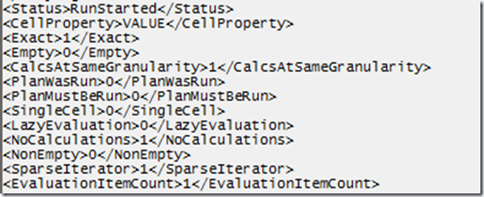
Here I have two fragments from the same evaluation node in Profiler.
I refer to the table for details about each tag. The most interesting here are:

  • · <Exact>1</Exact>: Which means that the subcube is an exact match.
  • · <LazyEvalutation>0</LazyEvaluation>: The evaluation node was run in bulked mode
  • · <SparseIterator>1</SparseIterator>: The evaluation node did not have to iterate over the entire cube. It was iterated over a smaller, sparse , space.

The collection of the tags i refer to are here.

InterestingTags1

InterestingTags2

Summary

This blog post is an introduction to evaluation nodes in SQL Server Profiler with the scenario of a cube with no calculations. This is why the resulting information from the profiler trace in this scenario is limited. The next post will have a look at evaluation nodes when MDX expressions are involved.

Table:Evaluation Node Tags

EvaluationNodeTag

Explanation

Exact

Exact means that the subcube is an exact match of the cells that are needed by the query. Sometimes the server can build a subcube that is *larger* than the cells needed by the query, and in that case Exact will be false.

Empty

Empty means that the result of this evaluation node is empty, none of the cells have any data . This can happen if you have a subcube that is somehow not valid (e.g. perhaps the subcube has a coordinate that doesn’t auto-exist with other coordinates or perhaps some other situation where calculations get eliminated until nothing remains and the subspace is guaranteed to have no cells with data).

PlanWasRun

PlanWasRun means the execution plan for this evaluation node has or has not yet been run. It will get run when the Run events show up – or it will *never* be run, because FE ends up fetching cell values in a cell-by-cell mode.

PlanMustBeRun

PlanMustBeRun is too internal to explain. But essentially there are some situations where we build an evaluation node, and it turns out that it matches another evaluation node that has already been executed – in that case, we can just point the evaluation node to the cached result of that earlier evaluation node, and the plan for the new evaluation node does not need to be run, and so the flag will be set to false.

NaiveEvaluation

This is on the evaluation node item. Use the value of the LazyEvaluation tag instead.

Status

PrePareStarted/Built/Uninitialized/RunStarted/RunSucceeded

CalcsAtSameGranularity

This indicates whether the calculations are on the same granularity or not.

SingleCell

This means whether the subcube of the evaluation node is for single cell coordinates. This may translate into cell-by-cell.

LazyEvaluation

Indicates cell-by-cell mode or bulk evaluation.

SparseIterator

When in block mode, do we have to iterate over the entire (dense) space of the entire subcube or can we iterate over a smaller (sparse) space. Remember that Sparse iteration is good. E.g. if you have a calculation with the expression [Measure1] * 2, and Measure1 is a storage engine measure, then we can execute a storage engine request and iterate just over the cells returned by the Storage engine request – which is a much sparser space than the entire subspace because many of the cell values are null and we don’t need to calculate them at all.

EvaluationItemCount

The number of calculations that apply to the subspace – these can change as we proceed through the stages of Init/Build/Prepare, because some of the calculations will get overlapped/split/eliminated. The final set is what you see at the end of Prepare or the beginning of Run

Overlaps

Overlaps means whether individual calculations overlap with each other. E.g. a scope on all states and a scope on the state of Washington – the item representing the first calculation has an overlapping calculation.

CoversFullSpace

CoversFullSpace means whether the calculation item covers the full space of the evaluation node, or whether the item has filters (e.g. State = Washington) that make it smaller than the full space of the evaluation node.

HasConditions

HasConditions refers to IF conditions in the calculations.

NoCalculations

0 -> Only Storage Engine Query

CellProperty

As discussed above.

CalculationLocation

This is the location of the calculation. When it is only SE queries this tag contains the measure group. In general it will contain the location and expression that applies to the evaluation node item.

VaryingAttributes

Drives the way the expression is evaluated and makes the expression dependant upon it. The 0s and 1s are bits and the numbers from 0 to 140 are the bits that are turned on .

Posted in Analysis Services SSAS | Tagged: , , | Leave a Comment »

Ancient Monument Spotting with Excel 2013 Data Explorer and Power View

Posted by thomasivarssonmalmo on April 14, 2013

While I am not working with BI or learning new technical stuff I read about archeology in Scandinavia and especially about what can be found in the region of Sweden where I live. One idea of mine is to be able to compare differnt types of acheological findings from different time periods and see if they appear on the same geographical spot or not. Can Excel 2013 help me with this? Yes it is possible with the help of Excel Data Explorer, currently in beta and PowerPivot and Power View.

First I need to show you the geographical spot so that you can relate to the area. I have highlighted one type of ancient monumnets in the Bing map that also shows the final result after this exercise. It is from Trelleborg municipality in south of Sweden since I have found a really good dataset from that part with a list of ancient monuments(stone age, bronze age and iron age). Most of these monuments are graves and burial mounds.


So where are we

The dataset can be found here on Wikipedia: http://sv.wikipedia.org/wiki/Lista_%C3%B6ver_fasta_fornminnen_i_Trelleborgs_kommun

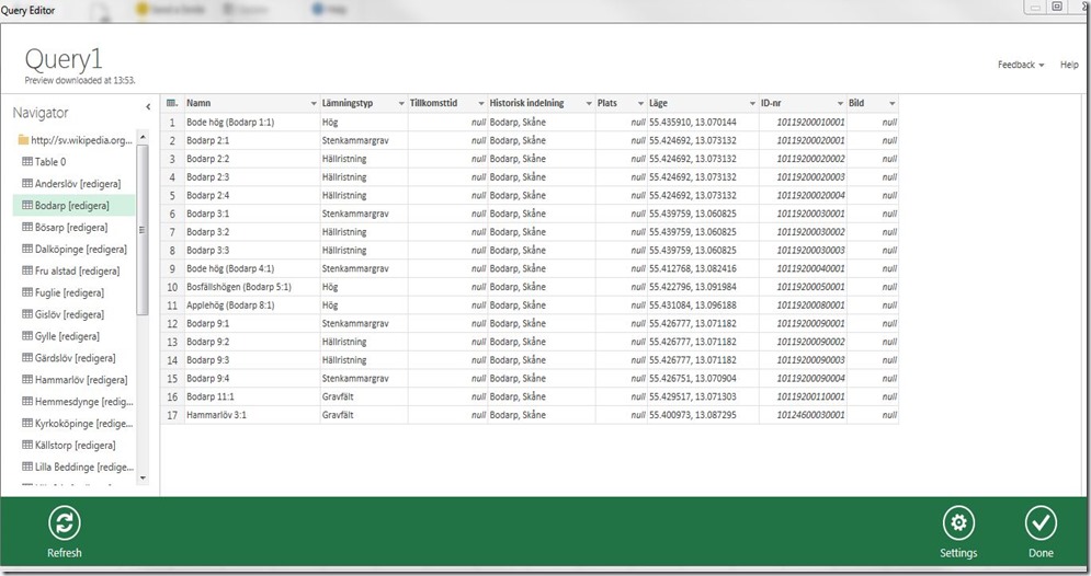
Below you can see how this Wiki-page looks like. Name is the unique registered number for each ancient monument. “Lämningstyp” is the classification like rune stones, burial mounds. “Historisk Indelning” is the actual geographic spot of the monument. “Läge” is the latitude and longitude of the monument and the key to map this information to the Bing Map in Power View.

The Data source

I started with launching Excel 2013 with the Data Explorer preview and selected from web as the data source. I simply added the url above and Data Explorer started the import. As you can see I got several datasets for different sub areas in Trelleborg. Here is an issue I have not solved yet and that is if I am able to import all data sets with one query by setting a parameter. With my approach I am able to show other steps in the cleaning and consolidation process with Data Explorer.


First Query

The cleaning process is straight forward. I have right clicked the columns I do not need and selected hide. I have also changed the data type of the Id-nr, a not important column, to text with the same righ click and quick menu. Finally I have added an Index column not for any specific reason that being able to run a count aggregation on that column. The final query result looks like this with the steps shown to the right.

cleaning steps

I have created one query for each different sub area within Trelleborg. With all queries defined I have used the Append button to add the sub areas to the same result set.


The appending process

This Append process is not the best way to run a union over all queries. It is possible to do this much quicker by changing the append query slightly. You simply add the query names to the function like you can see below.


Extend the query


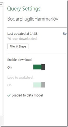
With this work done it is time to load the data into PowerPivot. In Excel 2013 this is done transparently and since I have only one single table there is no question about joins.


LoadToDataModel

After that I started Power View in Excel 2013(Insert)  the data model will appear. I select maps as the graphical tool in Power View. The selections for my map are the following. I need a measure in the size to see anything. I simply run a count on Lämningstyp(=classification of monument), and in Location I put the Latitude and Longitude data field. I added lämningstyp a second time for the color of the circles in Power View.


Selections for the map

The result look like this with two “Lämningstyp” selected in a filter. Gravfält is a burial field and Hög is a burial mound, usually from the bronze age. All sub areas are not loaded into the model so there are more monumnets than you see in the map.

Resulting Map

Below you also see the filter section.

The filter section


So what is the point of doing this? The is an available database together with maps of all ancient monuments in Sweden but without the flexibility of the Excel 2013 solution I have shown here. The fact that I can add colors to different groups or classification of monuments in Power View is very useful. It is possible to see different clusters of classifications on the same geographical spot or near by. I can also quickly select and unselect categories of monuments.

Posted in Excel 2013, Power View, PowerPivot and DAX | Tagged: , , | Leave a Comment »